Reference
- About This Guide
- I Advanced Administration
- II System
- 8 32-Bit and 64-Bit Applications in a 64-Bit System Environment
- 9 Booting a Linux System
- 10 The
systemdDaemon - 11
journalctl: Query thesystemdJournal - 12 The Boot Loader GRUB 2
- 13 Basic Networking
- 14 UEFI (Unified Extensible Firmware Interface)
- 15 Special System Features
- 16 Dynamic Kernel Device Management with
udev
- III Services
- IV Mobile Computers
- A An Example Network
- B GNU Licenses
5 Advanced Disk Setup
Sophisticated system configurations require specific disk setups. All
common partitioning tasks can be done with YaST. To get persistent
device naming with block devices, use the block devices below
/dev/disk/by-id or
/dev/disk/by-uuid. Logical Volume Management (LVM) is
a disk partitioning scheme that is designed to be much more flexible than
the physical partitioning used in standard setups. Its snapshot
functionality enables easy creation of data backups. Redundant Array of
Independent Disks (RAID) offers increased data integrity, performance, and
fault tolerance. openSUSE Leap also supports multipath I/O
, and there is also the option to use iSCSI as a
networked disk.
5.1 Using the YaST Partitioner #
With the expert partitioner, shown in Figure 5.1, “The YaST Partitioner”, manually modify the partitioning of one or several hard disks. You can add, delete, resize, and edit partitions, or access the soft RAID, and LVM configuration.
Warning: Repartitioning the Running System
Although it is possible to repartition your system while it is running, the risk of making a mistake that causes data loss is very high. Try to avoid repartitioning your installed system and always do a complete backup of your data before attempting to do so.
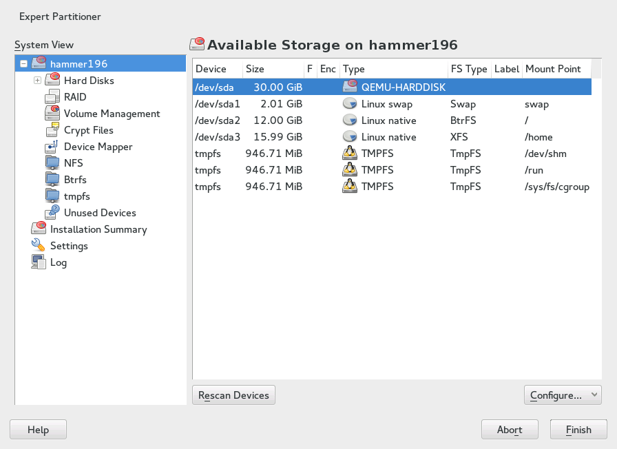
Figure 5.1: The YaST Partitioner #
All existing or suggested partitions on all connected hard disks are
displayed in the list of in the
YaST dialog. Entire hard disks
are listed as devices without numbers, such as
/dev/sda. Partitions are listed as parts
of these devices, such as
/dev/sda1. The size, type,
encryption status, file system, and mount point of the hard disks and
their partitions are also displayed. The mount point describes where the
partition appears in the Linux file system tree.
Several functional views are available on the left hand . Use these views to gather information about existing
storage configurations, or to configure functions like
RAID, Volume Management,
Crypt Files, or view file systems with additional
features, such as Btrfs, NFS, or TMPFS.
If you run the expert dialog during installation, any free hard disk space is also listed and automatically selected. To provide more disk space to openSUSE® Leap, free the needed space starting from the bottom toward the top of the list (starting from the last partition of a hard disk toward the first).
5.1.1 Partition Types #
Every hard disk has a partition table with space for four entries. Every entry in the partition table corresponds to a primary partition or an extended partition. Only one extended partition entry is allowed, however.
A primary partition simply consists of a continuous range of cylinders (physical disk areas) assigned to a particular operating system. With primary partitions you would be limited to four partitions per hard disk, because more do not fit in the partition table. This is why extended partitions are used. Extended partitions are also continuous ranges of disk cylinders, but an extended partition may be divided into logical partitions itself. Logical partitions do not require entries in the partition table. In other words, an extended partition is a container for logical partitions.
If you need more than four partitions, create an extended partition as the fourth partition (or earlier). This extended partition should occupy the entire remaining free cylinder range. Then create multiple logical partitions within the extended partition. The maximum number of logical partitions is 63, independent of the disk type. It does not matter which types of partitions are used for Linux. Primary and logical partitions both function normally.
Tip: GPT Partition Table
If you need to create more than 4 primary partitions on one hard disk, you need to use the GPT partition type. This type removes the primary partitions number restriction, and supports partitions bigger than 2 TB as well.
To use GPT, run the YaST Partitioner, click the relevant disk name in the and choose › › .
5.1.2 Creating a Partition #
To create a partition from scratch select and then a hard disk with free space. The actual modification can be done in the tab:
Select and specify the partition type (primary or extended). Create up to four primary partitions or up to three primary partitions and one extended partition. Within the extended partition, create several logical partitions (see Section 5.1.1, “Partition Types”).
Specify the size of the new partition. You can either choose to occupy all the free unpartitioned space, or enter a custom size.
Select the file system to use and a mount point. YaST suggests a mount point for each partition created. To use a different mount method, like mount by label, select . For more information on supported file systems, see
root.Specify additional file system options if your setup requires them. This is necessary, for example, if you need persistent device names. For details on the available options, refer to Section 5.1.3, “Editing a Partition”.
Click to apply your partitioning setup and leave the partitioning module.
If you created the partition during installation, you are returned to the installation overview screen.
5.1.2.1 Btrfs Partitioning #
The default file system for the root partition is Btrfs (see Chapter 3, System Recovery and Snapshot Management with Snapper for more information on Btrfs). The root file system is the default subvolume and it is not listed in the list of created subvolumes. As a default Btrfs subvolume, it can be mounted as a normal file system.
Important: Btrfs on an Encrypted Root Partition
The default partitioning setup suggests the root partition as Btrfs
with /boot being a directory. If you need to have the
root partition encrypted in this setup, make sure to use the GPT
partition table type instead of the default MSDOS type. Otherwise
the GRUB2 boot loader may not have enough space for the second stage loader.
It is possible to create snapshots of Btrfs subvolumes—either
manually, or automatically based on system events. For example when
making changes to the file system, zypper invokes the
snapper command to create snapshots before and after
the change. This is useful if you are not satisfied with the change
zypper made and want to restore the previous state.
As snapper invoked by zypper
snapshots the root file system by default, it is
reasonable to exclude specific directories from being snapshot,
depending on the nature of data they hold. And that is why YaST
suggests creating the following separate subvolumes.
Suggested Btrfs Subvolumes #
/tmp /var/tmp /var/runDirectories with frequently changed content.
/var/spoolContains user data, such as mails.
/var/libHolds dynamic data libraries and files plus state information pertaining to an application or the system.
By default, subvolumes with the option
no copy on
       write
are created for:/var/lib/mariadb,/var/lib/pgsql, and/var/lib/libvirt/images./var/logContains system and applications' log files which should never be rolled back.
/var/crashContains memory dumps of crashed kernels.
/srvContains data files belonging to FTP and HTTP servers.
/optContains third party software.
Tip: Size of Btrfs Partition
Because saved snapshots require more disk space, it is recommended to reserve more space for Btrfs partition than for a partition not capable of snapshotting (such as Ext3). Recommended size for a root Btrfs partition with suggested subvolumes is 20GB.
5.1.2.1.1 Managing Btrfs Subvolumes using YaST #
Subvolumes of a Btrfs partition can be now managed with the YaST module. You can add new or remove existing subvolumes.
Procedure 5.1: Btrfs Subvolumes with YaST #
Start the YaST with › .
Choose in the left pane.
Select the Btrfs partition whose subvolumes you need to manage and click .
Click . You can see a list off all existing subvolumes of the selected Btrfs partition. You can notice several
@/.snapshots/xyz/snapshotentries—each of these subvolumes belongs to one existing snapshot.Depending on whether you want to add or remove subvolumes, do the following:
To remove a subvolume, select it from the list of and click .
To add a new subvolume, enter its name to the text box and click .
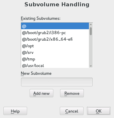
Figure 5.2: Btrfs Subvolumes in YaST Partitioner #
Confirm with and .
Leave the partitioner with .
5.1.3 Editing a Partition #
When you create a new partition or modify an existing partition, you can set various parameters. For new partitions, the default parameters set by YaST are usually sufficient and do not require any modification. To edit your partition setup manually, proceed as follows:
Select the partition.
Click to edit the partition and set the parameters:
- File System ID
Even if you do not want to format the partition at this stage, assign it a file system ID to ensure that the partition is registered correctly. Typical values are , , , and .
- File System
To change the partition file system, click and select file system type in the list.
openSUSE Leap supports several types of file systems. Btrfs is the Linux file system of choice for the root partition because of its advanced features. It supports copy-on-write functionality, creating snapshots, multi-device spanning, subvolumes, and other useful techniques. XFS, Ext3 and JFS are journaling file systems. These file systems can restore the system very quickly after a system crash, using write processes logged during the operation. Ext2 is not a journaling file system, but it is adequate for smaller partitions because it does not require much disk space for management.
The default file system for the root partition is Btrfs. The default file system for additional partitions is XFS.
Swap is a special format that allows the partition to be used as a virtual memory. Create a swap partition of at least 256 MB. However, if you use up your swap space, consider adding more memory to your system instead of adding more swap space.

Warning: Changing the File System
Changing the file system and reformatting partitions irreversibly deletes all data from the partition.
For details on the various file systems, refer to Storage Administration Guide.
- Encrypt Device
If you activate the encryption, all data is written to the hard disk in encrypted form. This increases the security of sensitive data, but reduces the system speed, as the encryption takes some time to process. More information about the encryption of file systems is provided in Book “Security Guide”, Chapter 11 “Encrypting Partitions and Files”.
- Mount Point
Specify the directory where the partition should be mounted in the file system tree. Select from YaST suggestions or enter any other name.
- Fstab Options
Specify various parameters contained in the global file system administration file (
/etc/fstab). The default settings should suffice for most setups. You can, for example, change the file system identification from the device name to a volume label. In the volume label, use all characters except/and space.To get persistent devices names, use the mount option , or . In openSUSE Leap, persistent device names are enabled by default.
If you prefer to mount the partition by its label, you need to define one in the text entry. For example, you could use the partition label
HOMEfor a partition intended to mount to/home.If you intend to use quotas on the file system, use the mount option . This must be done before you can define quotas for users in the YaST module. For further information on how to configure user quota, refer to Book “Start-Up”, Chapter 3 “Managing Users with YaST”, Section 3.3.4 “Managing Quotas”.
Select to save the changes.
Note: Resize File Systems
To resize an existing file system, select the partition and use . Note, that it is not possible to resize partitions while mounted. To resize partitions, unmount the relevant partition before running the partitioner.
5.1.4 Expert Options #
After you select a hard disk device (like ) in the pane, you can access the menu in the lower right part of the window. The menu contains the following commands:
- Create New Partition Table
This option helps you create a new partition table on the selected device.
Warning: Creating a New Partition Table
Creating a new partition table on a device irreversibly removes all the partitions and their data from that device.
- Clone This Disk
This option helps you clone the device partition layout (but not the data) to other available disk devices.
5.1.5 Advanced Options #
After you select the host name of the computer (the top-level of the tree in the pane), you can access the menu in the lower right part of the window. The menu contains the following commands:
- Configure iSCSI
To access SCSI over IP block devices, you first need to configure iSCSI. This results in additionally available devices in the main partition list.
- Configure Multipath
Selecting this option helps you configure the multipath enhancement to the supported mass storage devices.
5.1.6 More Partitioning Tips #
The following section includes a few hints and tips on partitioning that should help you make the right decisions when setting up your system.
Tip: Cylinder Numbers
Note, that different partitioning tools may start counting the cylinders
of a partition with 0 or with 1.
When calculating the number of cylinders, you should always use the
difference between the last and the first cylinder number and add one.
5.1.6.1 Using swap #
Swap is used to extend the available physical memory. It is then possible to use more memory than physical RAM available. The memory management system of kernels before 2.4.10 needed swap as a safety measure. Then, if you did not have twice the size of your RAM in swap, the performance of the system suffered. These limitations no longer exist.
Linux uses a page called “Least Recently Used” (LRU) to select pages that might be moved from memory to disk. Therefore, running applications have more memory available and caching works more smoothly.
If an application tries to allocate the maximum allowed memory, problems with swap can arise. There are three major scenarios to look at:
- System with no swap
The application gets the maximum allowed memory. All caches are freed, and thus all other running applications are slowed. After a few minutes, the kernel's out-of-memory kill mechanism activates and kills the process.
- System with medium sized swap (128 MB–512 MB)
At first, the system slows like a system without swap. After all physical RAM has been allocated, swap space is used as well. At this point, the system becomes very slow and it becomes impossible to run commands from remote. Depending on the speed of the hard disks that run the swap space, the system stays in this condition for about 10 to 15 minutes until the out-of-memory kill mechanism resolves the issue. Note that you will need a certain amount of swap if the computer needs to perform a “suspend to disk”. In that case, the swap size should be large enough to contain the necessary data from memory (512 MB–1GB).
- System with lots of swap (several GB)
It is better to not have an application that is out of control and swapping excessively in this case. If you use such application, the system will need many hours to recover. In the process, it is likely that other processes get timeouts and faults, leaving the system in an undefined state, even after terminating the faulty process. In this case, do a hard machine reboot and try to get it running again. Lots of swap is only useful if you have an application that relies on this feature. Such applications (like databases or graphics manipulation programs) often have an option to directly use hard disk space for their needs. It is advisable to use this option instead of using lots of swap space.
If your system is not out of control, but needs more swap after some time, it is possible to extend the swap space online. If you prepared a partition for swap space, add this partition with YaST. If you do not have a partition available, you can also use a swap file to extend the swap. Swap files are generally slower than partitions, but compared to physical RAM, both are extremely slow so the actual difference is negligible.
Procedure 5.2: Adding a Swap File Manually #
To add a swap file in the running system, proceed as follows:
Create an empty file in your system. For example, if you want to add a swap file with 128 MB swap at
/var/lib/swap/swapfile, use the commands:mkdir -p /var/lib/swap dd if=/dev/zero of=/var/lib/swap/swapfile bs=1M count=128
Initialize this swap file with the command
mkswap /var/lib/swap/swapfile

Note: Changed UUID for Swap Partitions when Formatting via
mkswapDo not reformat existing swap partitions with
mkswapif possible. Reformatting withmkswapwill change the UUID value of the swap partition. Either reformat via YaST (will update/etc/fstab) or adjust/etc/fstabmanually.Activate the swap with the command
swapon /var/lib/swap/swapfile
To disable this swap file, use the command
swapoff /var/lib/swap/swapfile
Check the current available swap spaces with the command
cat /proc/swaps
Note that at this point, it is only temporary swap space. After the next reboot, it is no longer used.
To enable this swap file permanently, add the following line to
/etc/fstab:/var/lib/swap/swapfile swap swap defaults 0 0
5.1.7 Partitioning and LVM #
From the , access the LVM configuration by clicking the item in the pane. However, if a working LVM configuration already exists on your system, it is automatically activated upon entering the initial LVM configuration of a session. In this case, all disks containing a partition (belonging to an activated volume group) cannot be repartitioned. The Linux kernel cannot reread the modified partition table of a hard disk when any partition on this disk is in use. If you already have a working LVM configuration on your system, physical repartitioning should not be necessary. Instead, change the configuration of the logical volumes.
At the beginning of the physical volumes (PVs), information about the
volume is written to the partition. To reuse such a partition for other
non-LVM purposes, it is advisable to delete the beginning of this volume.
For example, in the VG system and PV
/dev/sda2, do this with the command
dd if=/dev/zero of=/dev/sda2 bs=512
count=1.
Warning: File System for Booting
The file system used for booting (the root file system or
/boot) must not be stored on an LVM logical volume.
Instead, store it on a normal physical partition.
In case you want to change your /usr or
swap, refer to Procedure 9.1, “Updating Init RAM Disk When Switching to Logical Volumes”.
5.2 LVM Configuration #
This section briefly describes the principles behind the Logical Volume Manager (LVM) and its multipurpose features. In Section 5.2.2, “LVM Configuration with YaST”, learn how to set up LVM with YaST.
Warning: Back up Your Data
Using LVM is sometimes associated with increased risk such as data loss. Risks also include application crashes, power failures, and faulty commands. Save your data before implementing LVM or reconfiguring volumes. Never work without a backup.
5.2.1 The Logical Volume Manager #
The LVM enables flexible distribution of hard disk space over several file systems. It was developed because sometimes the need to change the segmenting of hard disk space arises just after the initial partitioning has been done. Because it is difficult to modify partitions on a running system, LVM provides a virtual pool (volume group, VG for short) of memory space from which logical volumes (LVs) can be created as needed. The operating system accesses these LVs instead of the physical partitions. Volume groups can occupy more than one disk, so that several disks or parts of them may constitute one single VG. This way, LVM provides a kind of abstraction from the physical disk space that allows its segmentation to be changed in a much easier and safer way than with physical repartitioning. Background information regarding physical partitioning can be found in Section 5.1.1, “Partition Types” and Section 5.1, “Using the YaST Partitioner”.
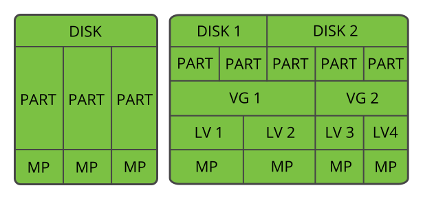
Figure 5.3: Physical Partitioning versus LVM #
Figure 5.3, “Physical Partitioning versus LVM” compares physical partitioning (left) with LVM segmentation (right). On the left side, one single disk has been divided into three physical partitions (PART), each with a mount point (MP) assigned so that the operating system can gain access. On the right side, two disks have been divided into two and three physical partitions each. Two LVM volume groups (VG 1 and VG 2) have been defined. VG 1 contains two partitions from DISK 1 and one from DISK 2. VG 2 contains the remaining two partitions from DISK 2. In LVM, the physical disk partitions that are incorporated in a volume group are called physical volumes (PVs). Within the volume groups, four LVs (LV 1 through LV 4) have been defined. They can be used by the operating system via the associated mount points. The border between different LVs do not need to be aligned with any partition border. See the border between LV 1 and LV 2 in this example.
LVM features:
Several hard disks or partitions can be combined in a large logical volume.
Provided the configuration is suitable, an LV (such as
/usr) can be enlarged if free space is exhausted.With LVM, it is possible to add hard disks or LVs in a running system. However, this requires hotpluggable hardware.
It is possible to activate a "striping mode" that distributes the data stream of an LV over several PVs. If these PVs reside on different disks, the read and write performance is enhanced, as with RAID 0.
The snapshot feature enables consistent backups (especially for servers) of the running system.
With these features, LVM is ready for heavily used home PCs or small servers. LVM is well-suited for the user with a growing data stock (as in the case of databases, music archives, or user directories). This would allow file systems that are larger than the physical hard disk. Another advantage of LVM is that up to 256 LVs can be added. However, working with LVM is different from working with conventional partitions. Instructions and further information about configuring LVM is available in the official LVM HOWTO at http://tldp.org/HOWTO/LVM-HOWTO/.
Starting from Kernel version 2.6, LVM version 2 is available, which is backward-compatible with the previous LVM and enables the continued management of old volume groups. When creating new volume groups, decide whether to use the new format or the backward-compatible version. LVM 2 does not require any kernel patches. It uses the device mapper integrated in kernel 2.6. This kernel only supports LVM version 2. Therefore, when talking about LVM, this section always refers to LVM version 2.
5.2.1.1 Thin Provisioning #
Starting from Kernel version 3.4, LVM supports thin provisioning. A thin-provisioned volume has a virtual capacity and a real capacity. Virtual capacity is the volume storage capacity that is available to a host. Real capacity is the storage capacity that is allocated to a volume copy from a storage pool. In a fully allocated volume, the virtual capacity and real capacity are the same. In a thin-provisioned volume, however, the virtual capacity can be much larger than the real capacity. If a thin-provisioned volume does not have enough real capacity for a write operation, the volume is taken offline and an error is logged.
For more general information, see http://wikibon.org/wiki/v/Thin_provisioning.
5.2.2 LVM Configuration with YaST #
The YaST LVM configuration can be reached from the YaST Expert Partitioner (see Section 5.1, “Using the YaST Partitioner”) within the item in the pane. The Expert Partitioner allows you to edit and delete existing partitions and also create new ones that need to be used with LVM. The first task is to create PVs that provide space to a volume group:
Select a hard disk from .
Change to the tab.
Click and enter the desired size of the PV on this disk.
Use and change the to . Do not mount this partition.
Repeat this procedure until you have defined all the desired physical volumes on the available disks.
5.2.2.1 Creating Volume Groups #
If no volume group exists on your system, you must add one (see Figure 5.4, “Creating a Volume Group”). It is possible to create additional groups by clicking in the pane, and then on . One single volume group is usually sufficient.
Enter a name for the VG, for example,
system.Select the desired . This value defines the size of a physical block in the volume group. All the disk space in a volume group is handled in blocks of this size.
Add the prepared PVs to the VG by selecting the device and clicking . Selecting several devices is possible by holding Ctrl while selecting the devices.
Select to make the VG available to further configuration steps.
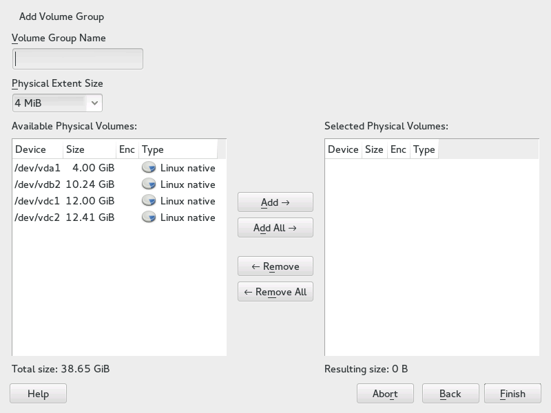
Figure 5.4: Creating a Volume Group #
If you have multiple volume groups defined and want to add or remove PVs, select the volume group in the list and click . In the following window, you can add or remove PVs to the selected volume group.
5.2.2.2 Configuring Logical Volumes #
After the volume group has been filled with PVs, define the LVs which the operating system should use in the next dialog. Choose the current volume group and change to the tab. , , , and LVs as needed until all space in the volume group has been occupied. Assign at least one LV to each volume group.
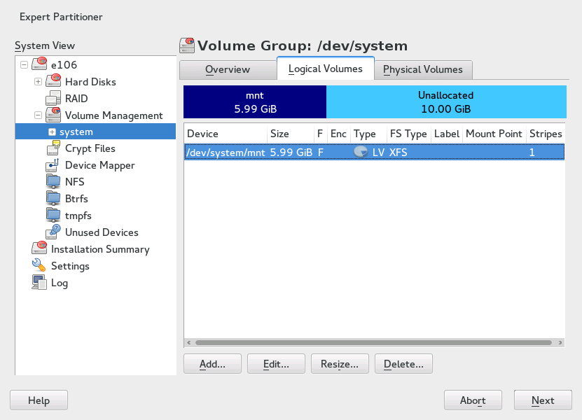
Figure 5.5: Logical Volume Management #
Click and go through the wizard-like pop-up that opens:
Enter the name of the LV. For a partition that should be mounted to
/home, a name likeHOMEcould be used.Select the type of the LV. It can be either , , or . Note that you need to create a thin pool first, which can store individual thin volumes. The big advantage of thin provisioning is that the total sum of all thin volumes stored in a thin pool can exceed the size of the pool itself.
Select the size and the number of stripes of the LV. If you have only one PV, selecting more than one stripe is not useful.
Choose the file system to use on the LV and the mount point.
By using stripes it is possible to distribute the data stream in the LV among several PVs (striping). However, striping a volume can only be done over different PVs, each providing at least the amount of space of the volume. The maximum number of stripes equals to the number of PVs, where Stripe "1" means "no striping". Striping only makes sense with PVs on different hard disks, otherwise performance will decrease.
Warning: Striping
YaST cannot, at this point, verify the correctness of your entries concerning striping. Any mistake made here is apparent only later when the LVM is implemented on disk.
If you have already configured LVM on your system, the existing logical volumes can also be used. Before continuing, assign appropriate mount points to these LVs. With , return to the YaST Expert Partitioner and finish your work there.
5.3 Soft RAID Configuration #
The purpose of RAID (redundant array of independent disks) is to combine several hard disk partitions into one large virtual hard disk to optimize performance and/or data security. Most RAID controllers use the SCSI protocol because it can address a larger number of hard disks in a more effective way than the IDE protocol. It is also more suitable for the parallel command processing. There are some RAID controllers that support IDE or SATA hard disks. Soft RAID provides the advantages of RAID systems without the additional cost of hardware RAID controllers. However, this requires some CPU time and has memory requirements that make it unsuitable for high performance computers.
With openSUSE® Leap , you can combine several hard disks into one soft RAID system. RAID implies several strategies for combining several hard disks in a RAID system, each with different goals, advantages, and characteristics. These variations are commonly known as RAID levels.
Common RAID levels are:
- RAID 0
This level improves the performance of your data access by spreading out blocks of each file across multiple disk drives. Actually, this is not really a RAID, because it does not provide data backup, but the name RAID 0 for this type of system is commonly used. With RAID 0, two or more hard disks are pooled together. Performance is enhanced, but the RAID system is destroyed and your data lost if even one hard disk fails.
- RAID 1
This level provides adequate security for your data, because the data is copied to another hard disk 1:1. This is known as hard disk mirroring. If one disk is destroyed, a copy of its contents is available on the other one. All disks but one could be damaged without endangering your data. However, if the damage is not detected, the damaged data can be mirrored to the undamaged disk. This could result in the same loss of data. The writing performance suffers in the copying process compared to using single disk access (10 to 20 % slower), but read access is significantly faster in comparison to any one of the normal physical hard disks. The reason is that the duplicate data can be parallel-scanned. Generally it can be said that Level 1 provides nearly twice the read transfer rate of single disks and almost the same write transfer rate as single disks.
- RAID 5
RAID 5 is an optimized compromise between Level 0 and Level 1, in terms of performance and redundancy. The hard disk space equals the number of disks used minus one. The data is distributed over the hard disks as with RAID 0. Parity blocks, created on one of the partitions, exist for security reasons. They are linked to each other with XOR, enabling the contents to be reconstructed by the corresponding parity block in case of system failure. With RAID 5, no more than one hard disk can fail at the same time. If one hard disk fails, it must be replaced as soon as possible to avoid the risk of losing data.
- RAID 6
To further increase the reliability of the RAID system, it is possible to use RAID 6. In this level, even if two disks fail, the array still can be reconstructed. With RAID 6, at least 4 hard disks are needed to run the array. Note that when running as software raid, this configuration needs a considerable amount of CPU time and memory.
- RAID 10 (RAID 1+0)
This RAID implementation combines features of RAID 0 and RAID 1: the data is first mirrored to separate disk arrays, which are inserted into a new RAID 0; type array. In each RAID 1 sub-array, one disk can fail without any damage to the data. A minimum of four disks and an even number of disks is needed to run a RAID 10. This type of RAID is used for database application where a huge load is expected.
- Other RAID Levels
Several other RAID levels have been developed (RAID 2, RAID 3, RAID 4, RAIDn, RAID 10, RAID 0+1, RAID 30, RAID 50, etc.), some being proprietary implementations created by hardware vendors. These levels are not very common and therefore are not explained here.
5.3.1 Soft RAID Configuration with YaST #
The YaST configuration can be reached from the YaST Expert Partitioner, described in Section 5.1, “Using the YaST Partitioner”. This partitioning tool enables you to edit and delete existing partitions and create new ones to be used with soft RAID:
Select a hard disk from .
Change to the tab.
Click and enter the desired size of the raid partition on this disk.
Use and change the to . Do not mount this partition.
Repeat this procedure until you have defined all the desired physical volumes on the available disks.
For RAID 0 and RAID 1, at least two partitions are needed—for RAID 1, usually exactly two and no more. If RAID 5 is used, at least three partitions are required, RAID 6 and RAID 10 require at least four partitions. It is recommended to use partitions of the same size only. The RAID partitions should be located on different hard disks to decrease the risk of losing data if one is defective (RAID 1 and 5) and to optimize the performance of RAID 0. After creating all the partitions to use with RAID, click › to start the RAID configuration.
In the next dialog, choose between RAID levels 0, 1, 5, 6 and 10. Then, select all partitions with either the “Linux RAID” or “Linux native” type that should be used by the RAID system. No swap or DOS partitions are shown.
Tip: Classify Disks
For RAID types where the order of added disks matters, you can mark individual disks with one of the letters A to E. Click the button, select the disk and click of the buttons, where X is the letter you want to assign to the disk. Assign all available RAID disks this way, and confirm with . You can easily sort the classified disks with the or buttons, or add a sort pattern from a text file with .
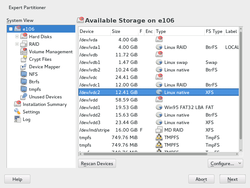
Figure 5.6: RAID Partitions #
To add a previously unassigned partition to the selected RAID volume, first click the partition then . Assign all partitions reserved for RAID. Otherwise, the space on the partition remains unused. After assigning all partitions, click to select the available .
In this last step, set the file system to use, encryption and
the mount point for the RAID volume. After completing the configuration
with , see the /dev/md0
device and others indicated with RAID in the expert
partitioner.
5.3.2 Troubleshooting #
Check the file /proc/mdstat to find out whether a
RAID partition has been damaged. If th system fails, shut
down your Linux system and replace the defective hard disk with a new one
partitioned the same way. Then restart your system and enter the command
mdadm /dev/mdX --add /dev/sdX. Replace 'X' with your
particular device identifiers. This integrates the hard disk
automatically into the RAID system and fully reconstructs it.
Note that although you can access all data during the rebuild, you may encounter some performance issues until the RAID has been fully rebuilt.
5.3.3 For More Information #
Configuration instructions and more details for soft RAID can be found in the HOWTOs at:
/usr/share/doc/packages/mdadm/Software-RAID.HOWTO.html
Linux RAID mailing lists are available, such as http://marc.info/?l=linux-raid.